Gaussian Graph Convolutional Networks
I’m using graph convolutional networks as a tool to segment the cortical surface of the brain. This research resides in the domain of node classification using inductive learning. By node classification, I mean that we wish to assign a discrete label to cortical surface locations (nodes / vertices in a graph) on the basis of some feature data and brain network topology. By inductive learning, I mean that we will train, validate, and test on datasets with possibly different graph topologies – this is in contrast to transductive learning that learns models that do not generalize to arbitrary network topology.
In conventional convolutions over regular grid domains, such as images, using approaches like ConvNet, we learn the parameters of a sliding filter that convolves the signal around a pixel of interest $p_{i,j}$, such that we aggregate the information from pixels $p_{\Delta i, \Delta j}$ for some fixed distance $\Delta$ away from $p$. Oftentimes, however, we encounter data that is distributed over a graphical domain, such as social networks, journal citations, brain connectivity, or the electrical power grid. In such cases, concepts like “up”, “down”, “left”, and “right” do not make sense – what does it mean to be “up” from something in a network? – so we need some other notion of neighborhood.
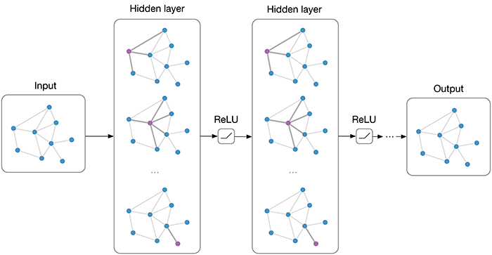
In come graph convolutional networks (GCNs). GCNs generalize the idea of neighborhood aggregation to the graph domain by utilizing the adjacency structure of a network – we can now aggregate signals near a node by using some neighborhood around it. While vanilla GCNs learn rotationally-invariant filters, recent developments in the world of Transformer networks have opened up the door for much more flexible and inductive models (see: Graph Attention Networks, GraphSAGE).
I was specifically interested in applying the methodology described here, where the authors utilitize Gaussian kernels as filters over the neighborhood of nodes. However, the authors did not open-source their code – as such, I needed to implement this method myself. Assume our input data to layer $l$ is $Y^{(l)} \in \mathbb{R}^{N \times q}$ for $N$ nodes in the graph. We can define the Gaussian kernel-weighted convolution as follows:
$$ \begin{align} z_{i,p}^{(l)} = \sum_{j \in \mathcal{N}_{i}} \sum_{q=1}^{M_{(l)}} \sum_{k=1}^{K_{(l)}} w_{p,q,k}^{(l)} \cdot y_{j,q}^{(l)} \cdot \phi(\hat{\mu}_{i}, \hat{\mu}_{j}; \Theta_{k}^{(l)}) + b_{p}^{(l)} \end{align} $$
Above, $y_{j,q}^{(l)}$ is the $q$-th input feature of neighboring node $j$, $w_{p,q,k}^{(l)}$ is the linear weight assigned to this feature for the $k$-th kernel, and $\phi(\hat{\mu}_{i}, \hat{\mu}_{j}; \Theta_{k}^{(l)})$ is the $k$-th kernel weight between node $i$ and node $j$, defined as:
$$ \begin{align} \phi(\hat{\mu_{i}}, \hat{\mu_{j}}; \sigma_{k}^{(l)}, \mu_{k}^{(l)} ) = \exp^{-\sigma_{k}^{(l)} \left\Vert (\hat{\mu_{i}} - \hat{\mu_{j}}) - \mu_{k}^{(l)} \right\Vert^{2}} \end{align} $$
Extrinsically, the kernel weights are represented by edges in a sparse affinity matrix, such that index $(i,j)$ is the Gaussian kernel weight between node $i$ and node $j$ for the $k$-th kernel in the $l$-th layer, where nodes $j$ are restricted to be within a certain neighborhood or distance of node $i$. This can be seen more clearly here:

I implemented a new convolutional layer called GAUSConv (available
here). To implement this algorithm, I utilized the
Deep Graph Library (DGL), which offers a stellar single unifed API based on message passing (I’m using
Pytorch as the backend). I noticed that I could formulate this problem using attention mechanisms described in the
Graph Attention Network paper – however, instead of computing attention weights using a fully connected layer as described in that work, I would compute kernel weights using Gaussian filters. Similarly, just as the GAT paper describes multi-head attention for multiple attention channels, I could analogize my fomulation to multi-head kernels for multiple kernel channels. To this end, I could make use of the
GATConv API quite easily by replacing the attention computations with the Gaussian kernel filtrations. Likewise, I utilized the
GraphConv API to incorporate linear weights from the
Graph Convolution Network paper.
The GAUSConv layer is similar to both the GraphConv and GATConv layers but differs in a few places. Rather than initializing the layer with attention heads, we initialize it with the number of kernels and a kernel dropout probability.
GAUSConv(in_feats, # number of input dimensions
         out_feats, # number of output features
         num_kernels, # number of kernels for current layer
         feat_drop=0., # dropout probability of features
         kernel_drop=0., # dropout probability of kernels
         negative_slope=0.2, # leakly relu slope
         activation=None, # activation function to apply after forward pass
         random_seed=None, # for example / reproducibility purposes
         allow_zero_in_degree=False)
Importantly, in the layer instantiation, we define linear weights and kernel mean and sigma parameters, mu and sigma. We initialize both kernel parameters with the flag require_grad=True, which enables us to update these kernel parameters during the backward pass of the layer. Both parameters are initialized with values in the reset_parameters method.
# initialize feature weights and bias vector
self.weights = nn.Parameter(
    th.Tensor(num_kernels, in_feats, out_feats), requires_grad=True)
self.bias = nn.Parameter(
    th.Tensor(num_kernels, out_feats), requires_grad=True)

# initialize kernel perameters
self.mu = nn.Parameter(
    th.Tensor(1, num_kernels, in_feats), requires_grad=True)
self.sigma = nn.Parameter(
    th.Tensor(num_kernels, 1), requires_grad=True)
Now here is the clever part, and where the
DGL message passing interface really shines through. DGL fuses the send and receive messages so that no messages between nodes are ever explicitly stored, using built-in message and reduce functions. To compute the kernel weights between all pairs of source and destrination nodes, we use these built-in functions. The important steps are:
compute node feature differences between all source / destination node pairs
aggregate and reduce incoming messages from destination nodes scaled by the kernel weights, to update the source node features
In the forward pass of our layer, we perform the following steps:
### forward pass of GAUSConv layer ###

# compute all pairwise differences between adjacent node features
graph.ndata['h'] = feat
graph.apply_edges(fn.u_sub_v('h', 'h', 'diff'))

# compute kernel weights for each source / desintation pair
e = graph.edata['diff'].unsqueeze(1) - mu
e = -1*sigma*th.norm(e, dim=2).unsqueeze(2)
e = e.exp()
graph.edata['e'] = e

# apply kernel weights to destination node features
graph.apply_edges(fn.v_mul_e('h', 'e', 'kw'))

# apply linear projection to kernel-weighted destination node features
a = th.sum(th.matmul(graph.edata['kw'].transpose(1, 0), weights), dim=0)

# apply kernel dropout
a = self.kernel_drop(a)
graph.edata['a'] = a

# final message-passing and reduction step
# aggregate weighted destination node features to update source node features
graph.update_all(fn.copy_e('a', 'm'), fn.sum('m', 'h'))
rst = graph.ndata['h']
As an example, given a graph and features, we instantiate a GAUSConv layer and propogate our features through the network via:
# set random seed
random_seed=1

# define arbitrary input/output feature shape
n_samples = 4
in_feats=4
out_feats=2
features = th.ones(n_samples, in_feats)

# define number of kernels
num_kernels=2

# create graph structure
u, v = th.tensor([0, 0, 0, 1]), th.tensor([1, 2, 3, 3])
g = dgl.graph((u, v))
g = dgl.to_bidirected(g)
g = dgl.add_self_loop(g)

# instantiate layer
GausConv = GAUSConv(in_feats=in_feats,
                    out_feats=out_feats,
                    random_seed=random_seed,
                    num_kernels=num_kernels,
                    feat_drop=0,
                    kernel_drop=0)

# forward pass of layer
logits = GausConv(g, features)

print(logits)
tensor([[0.1873, 0.7217],
        [0.1405, 0.5413],
        [0.0936, 0.3608],
        [0.1405, 0.5413]], grad_fn=<AddBackward0>)