fieldmodel

This is a Python package for fitting densities to scalar fields distributed on the domain of regular meshes. This package is an implementation of the methodology described here. Rather than using the spatial coordinates of the mesh on which the data is distributed, this package fits isotropic distributions using the geodesic distances between mesh vertices.

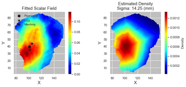
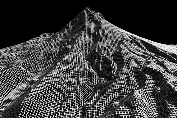
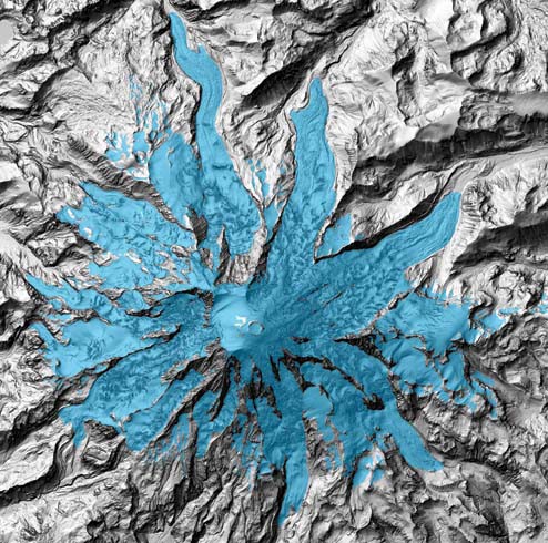
Given a scalar field assigning, let’s say, elevation values to latitude-longitude coordinates of Mount Rainier, we could use fieldmodel to fit a Gaussian distribution to this elevation profile. The output of this fitting procedure would be 2 parameters: a mean parameter (centered on the true summit coordinates) and a sigma parameter, a measure of how quickly the elevation profile decays as we move away from the summit.

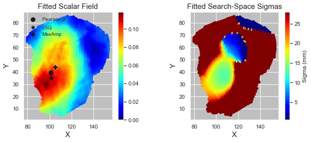
The code iterates over all possible mean locations in a set, and optimizes the sigma parameter using a BFGS minimization procedure. I provide 3 optimality criteria options:

1. maximization of spatial correlation
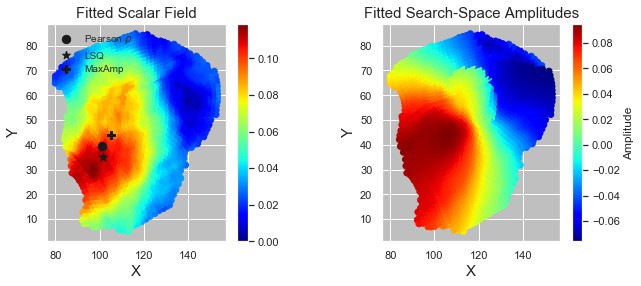
2. maximization of signal amplitude
3. minimization of least-squares error

Along with fitting procedure, fieldmodel also offers some basic plotting functionality to visualize the fitted densities alongside the data to which those densities were fit.

How to install and use:

git clone https://github.com/kristianeschenburg/fieldmodel.git
cd  ./fieldmodel
pip install .

Example application to synthetic data:

import numpy as np
import scipy.io as sio

# Create fake distance matrix between and fake scalar map

# x coordinates for plotting
tx_file = '../data/target.X.mat'
tx = sio.loadmat(tx_file)['x'].squeeze()

# y coordinates for plotting
ty_file = '../data/target.Y.mat'
ty = sio.loadmat(ty_file)['y'].squeeze()

# geodesic distance matrix between vertices
dist_file = '../data/distance.mat'
dist = sio.loadmat(dist_file)['apsp']

# scalar field
field_file = '../data/scalar_field.mat'
field = sio.loadmat(field_file)['field'].squeeze()

Next, we can instantiate and fit our fieldmodel. For more detail on the parameters, please refer to the docstring or Demo.ipynb in the demos directory.

from fieldmodel import GeodesicFieldModel as GFM

# instantiate field model
G = GFM.FieldModel(r=10, amplitude=False,
                    peak_size=15, hood_size=20,
                    verbose=False, metric='pearson')

# fit field model
G.fit(data=field, distances=dist, x=tx, y=ty)

We can visualize the results of our model via the plot method in GFM.fieldmodel:

G.plot(field='pdf')
G.plot(field='amplitude')
G.plot(field='sigma')