Distances Between Subspaces

I’m working with some multi-dimensional float-valued data – I’ll call a single instance of this data $X \in \mathbb{R}^{n \times k}$. I have multiple samples $X_{1}, X_{2}…X_{t}$, and want to compare these subspaces – namely, I want to compute the distance between pairs of subspaces.

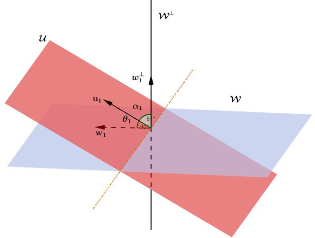
Let’s assume that our subspaces are not rank-deficient – i.e. for a given subspace sample, all of our dimensions are linearly independent. Thus, the $k$ vectors form a basis set that spans some $k$-d subspace in $\mathbb{R}^{n}$. We can think of each $k$-d subspace as a hyperplane in $(k+1)$-d space, just as we can think of a 2-d plane in 3-d space. One way to compare these subspaces is by using the “principle angles between subspaces” (or angles between flats). We can compare the “angles” between these hyperplanes, which will tell us how “far apart” the two subspaces are.

This comparison is effectively based on the QR decomposition and the Singular Value Decomposition. For two subspaces $[U, W]$, we compute the QR decomposition of both:

$$\begin{align} U &= Q_{u}R_{u}\\
W &= Q_{w}R_{w}\\
\end{align}$$

where $Q_{u}$ and $Q_{w} \in \mathbb{R}^{n \times k}$ are orthonormal bases such that $Q_{u}^{T}Q_{u} = Q_{w}^{T}Q_{w} = I_{k}$ that span the same subspace as the original columns of $U$ and $W$, and $R_{u}$ and $R_{w} \in \mathbb{R}^{k \times k}$ are lower triangular matrices. Next, we compute the matrix $D = \langle Q_{u}, Q_{w} \rangle = Q_{u}^{T} Q_{w} \in \mathbb{R}^{k \times k}$, and then apply the singular value decomposition:

$$\begin{align} D = USV^{T} \end{align}$$

We can sort of think of $D$ as the cross-covariance matrix. As such, the singular vectors represent the main orthogonal axes of cross-covariation between our two subspaces, while the singular values represent angles. In order to compute the principle angles of our subspaces, we simply take

$$\begin{align} \theta &= cos^{-1}(S) \\
&=cos^{-1}[\sigma_{1}, \sigma_{2}…\sigma_{k}] \end{align}$$

which gives us the principle angles (in radians). Because the SVD is invariant to sign (+/-), the principle angles range between $\Big[0, \frac{\pi}{2}\Big]$. This means that subspaces that span the same space have a principle angle of 0, and subspaces that are orthogonal (maximally far apart) to one another have a principle angle of $\frac{\pi}{2}$.

In order to compute the “distance” between our subspaces, we can apply various metrics to our vector of principle angles. The simplest approach is to apply the $L2$ norm to our vector of principle angles, $\theta$, as

$$\begin{align} d(X_{i}, X_{j}) = \sqrt{\sum_{n=1}^{k} cos^{-1}(\sigma_{n})^{2}} \end{align}$$

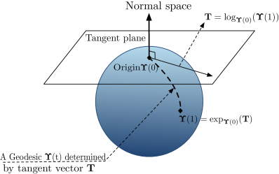
This metric is called the Grassmann Distance and is formally related to the geodesic distance between subspaces distributed on the Grassmannian manifold.

This, however, is a topic for another future blog post. There are a variety of metrics we can use to compute the pairwise distance between subspaces, some of which are

• Asimov: $\; max(\theta)$
• Fubini-Study: $\; cos^{-1}(\prod sin(\theta))$
• Spectral: $\; 2 sin(\frac{max(\theta)}{2})$

but all are fundamentally based on some function of our vector of principle angles, $\theta$.